Response of driven weakly chaotic systems
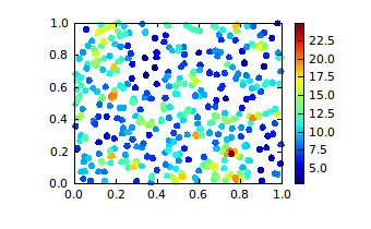
Mott random site model
In this model, the sites are randomly distributed in space, and the rates depend on the distance between sites: \[ w_{nm} \ \ =\ \ w_0 \cdot \exp\left(-\frac{\left|r_n-r_m\right|}{\xi} - \epsilon_{nm}\right)\] Where \(\xi\) and \(w_0\) are system parameters (defining the time and space units), and \(\epsilon\) a bond specific parameter. In the degenerate version, \(\epsilon=0\) for all the bonds, while in the non-degenerate version \(\epsilon_{nm} = \textrm{uniform}[0,\infty]\).The dimensionless parameter defining sparsity in this model is \[ s \ \ =\ \ \frac{\xi}{r_0} \] where \(r_0\) is the typical distance between sites.
Determining the diffusion coefficient \(D\)
The long term behavior of the system is characterized by
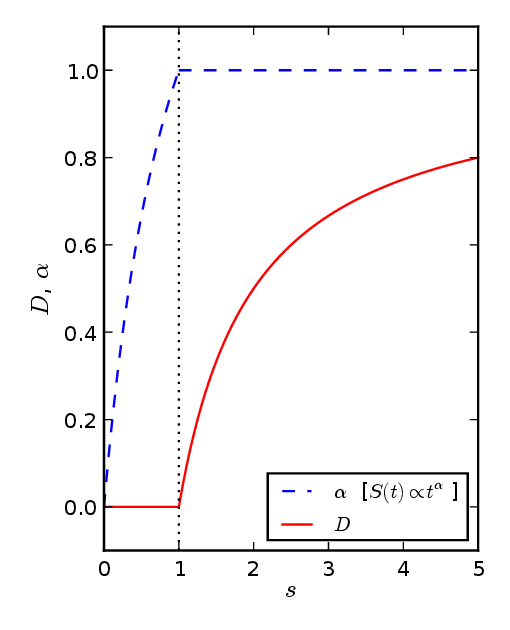
a diffusion coefficient \(D\). It is defined by the long term spreading:
\[ S(t)\quad = \quad \left\langle r^2(t)\right\rangle \quad \sim \quad D t\]
And it is also related to the long time survival probability:
\[ \mathcal{P}(t)\quad \sim \quad \frac{1}{(Dt)^{1/2}} \]
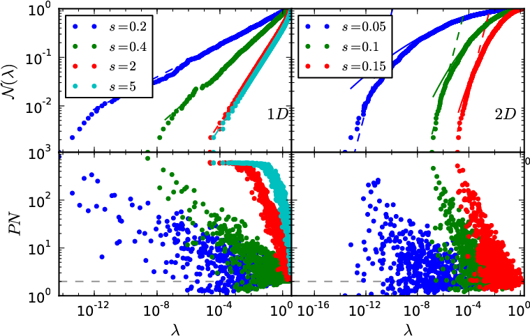
And to the low eigenvalue distribution (by Laplace transform):
\[ \mathcal{N}(\lambda) \quad \sim \quad \left[ \frac{\lambda}{D}\right]^{d/2} \]

Effective range hopping
For a dense system, (large \(\xi\) compared to typical site distance), the diffusion coefficient can be estimated by a linear equation (linear in the rates): \[ D_{\textrm{linear}} = \frac{1}{2d}\sum_r w(r) r^2 \] We present the ERH procedure to estimate \(D\), based on resistor network analysis, with a smooth cross-over between the dense and sparse regimes.
Results for the degenerate model
\[ D \quad =\quad \textrm{EXP}_{d+2}\left(\frac{1}{s_\textrm{eff}}\right) \mbox{e}^{-1/s_\textrm{eff}} D_{\textrm{linear}} \\ s_\textrm{eff}\quad=\quad \left(\frac{d}{\Omega_d} n_c\right)^{-1/d}\frac{\xi}{r_0} \\ \textrm{EXP}_{l}(x) \quad = \quad \sum_{k=0}^l \frac{1}{k!}x^k\]
- The parameter \(n_c\) is the average number of bonds required to get percolation. For \(d=1\) \(n_c=2\) and for \(d=2\) \(n_c\approx 4.5\), based on studies of disk-percolation.
- If we disregard the percolative nature (by setting \(n_c=0\)), we get the linear estimate back.
- In the limit \(s_\textrm{eff}\ll 1\) we obtain VRH-like behavior: \[ D\sim e^{-1/s_\textrm{eff}} \]
Results for the non-degenerate "Mott" model
In this case, \(s_\textrm{eff}\) depends explicitly on the temperature, i.e.: \[s_{\textrm{eff}}\quad=\quad \left(\frac{d}{\Omega_d} n_c \left(\frac{T}{\Delta_\xi}\right)\right)^{-1/(d+1)} \] Where \(\Delta_\xi\) is the mean level spacing. Apart from that, the only change in \(D\) is the polynomial order: \[ D \quad =\quad \textrm{EXP}_{\color{red}{d+3}}\left(\frac{1}{s_{\textrm{eff}}}\right) \mbox{e}^{-1/s_{\textrm{eff}}} D_{linear} \] In the limit \(s\ll 1\), we get the familiar VRH estimate that has been presented long ago by Nevill Francis Mott. \[ D \sim \left(\frac{1}{T}\right)^{2/(d+1)} \exp\left[-\left(\frac{T_0}{T}\right)^{1/(d+1)}\right]\]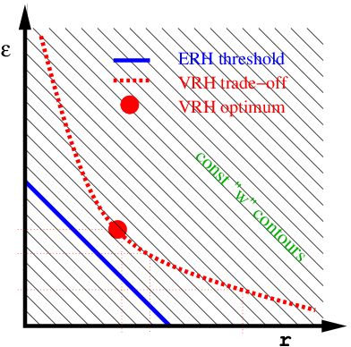
Diffusion in sparse networks: linear to semi-linear crossover [arXiv] [pdf],
Y. de Leeuw, D. Cohen, Phys. Rev. E 86, 051120 (2012).